[PyTorch] Multivariable Linear Regression 실습 : 모두를 위한 딥러닝 시즌2

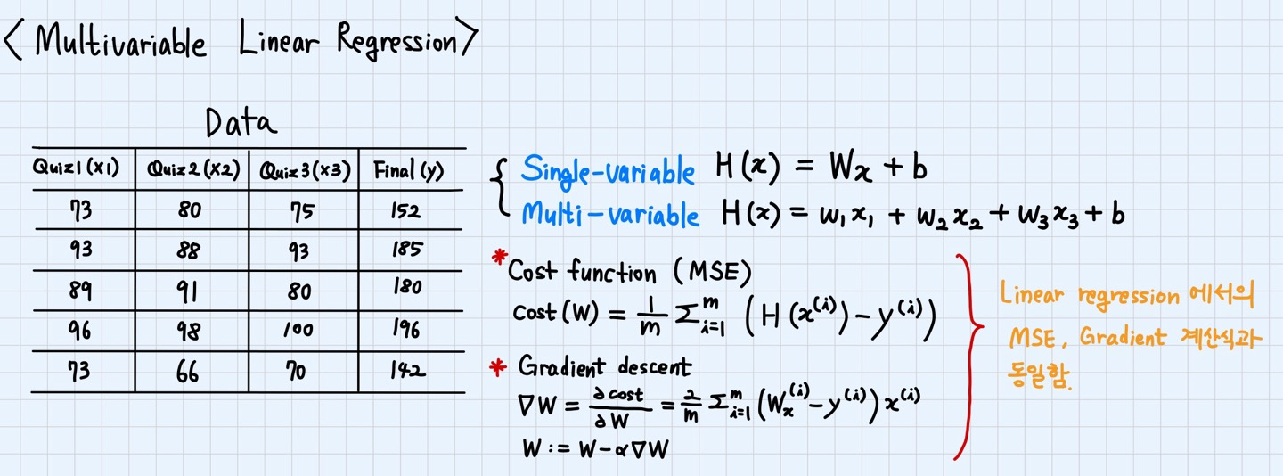
Multivariable Linear Regression 이론 요약

 Linear regression과 Multivariable Linear Regression의 Hypothesis 식은 변수의 개수로 인해 차이가 있으나, Cost function 및 Gradient 계산식은 동일하게 적용된다.

Multivariable Linear Regression 구현 코드

 모델 생성과 Hypothesis 및 Cost 계산을 직접 수행하는 방식과 모듈 및 함수를 활용하는 방식 2가지로 구현을 했다.

 

방법 1. W, b로 모델 생성 & 직접 Cost 계산

import torch
import torch.optim as optim

# Data definition
x_train = torch.FloatTensor([[73, 80, 75],
                            [93, 88, 93],
                            [89, 91, 90],
                            [96, 98, 100],
                            [73, 66, 70]])
y_train = torch.FloatTensor([[152], [185], [180], [196], [142]])

# Initialize model
W = torch.zeros((3,1), requires_grad=True)
b = torch.zeros(1, requires_grad=True)

# Optimization definition
optimizer = optim.SGD([W, b], lr=1e-5)

nb_epochs = 20
for epoch in range(nb_epochs + 1):
    
    # Calculate H(x)
    hypothesis = x_train.matmul(W) + b # or .mm or @
    
    # Calculate Cost
    cost = torch.mean((hypothesis - y_train) ** 2)
    
    # Gradient Descent
    optimizer.zero_grad()
    cost.backward()
    optimizer.step()
    
    print('Epoch {:4d}/{} hypothesis: {} Cost: {:.6f}'.format(
        epoch, nb_epochs, hypothesis.squeeze().detach(), cost.item()
    ))

 

방법 2. nn.Module을 상속해서 모델 생성 & mse_loss 함수로 Cost 계산

import torch
import torch.optim as optim
import torch.nn as nn
import torch.nn.functional as F

class MultivariateLinearRegressionModel(nn.Module):
    def __init__(self):
        super().__init__()
        self.linear = nn.Linear(3, 1)  # 3 Input, 1 Output
        
    def forward(self, x):
        return self.linear(x)
    
# Data definition
x_train = torch.FloatTensor([[73, 80, 75],
                            [93, 88, 93],
                            [89, 91, 90],
                            [96, 98, 100],
                            [73, 66, 70]])
y_train = torch.FloatTensor([[152], [185], [180], [196], [142]])

# Initialize model
model = MultivariateLinearRegressionModel()

# Optimization definition
optimizer = optim.SGD(model.parameters(), lr=1e-5)

nb_epochs = 20
for epoch in range(nb_epochs + 1):
    
    # Calculate H(x)
    hypothesis = model(x_train)
    
    # Calculate Cost
    cost = F.mse_loss(hypothesis, y_train)
    
    # Gradient Descent
    optimizer.zero_grad()
    cost.backward()
    optimizer.step()
    
    print('Epoch {:4d}/{} hypothesis: {} Cost: {:.6f}'.format(
        epoch, nb_epochs, hypothesis.squeeze().detach(), cost.item()
    ))

실행 결과 분석

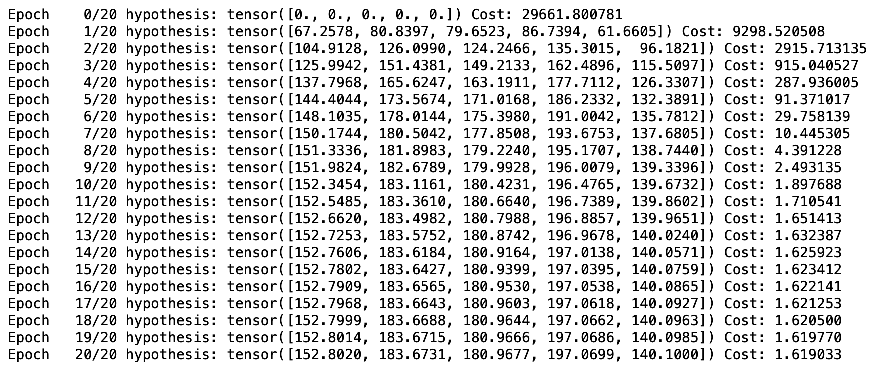
[방법 1 실행 결과] H(x)는 점점 y에 가까워지며, Cost는 점점 작아진다.

 

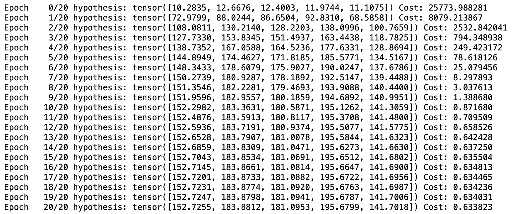
[방법 2 실행 결과] Epoch가 증가할 때마다, 방법 1과 동일한 방향성을 가지고 값이 업데이트되었다. 단, 방법 1에 비해 방법2를 사용했을 때, H(x)가 조금 더 y에 가깝고 Cost도 훨씬 작게 나타났다.

느낀 점

•  W, b를 정의한 후에  optimizer 정의, H(x) 및 Cost 계산에 사용하는 방법을 통해서 각각의 연산 단계가 의미하는 바를 정확히 이해할 수 있어서 좋았다.
• 그러나 nn.Module을 상속받아 사용하거나, mse_loss와 같은 함수를 사용하는 것이 성능도 더 좋고, 편리한 것 같다. 

 

*참고 자료

모두를 위한 딥러닝 시즌2 - [PyTorch] Lab-04-1 Multivariable Linear regression

https://youtu.be/1JT8KhvymmY?feature=shared