[PyTorch] Perceptron & Multi Layer Perceptron 실습 : 모두를 위한 딥러닝 시즌2

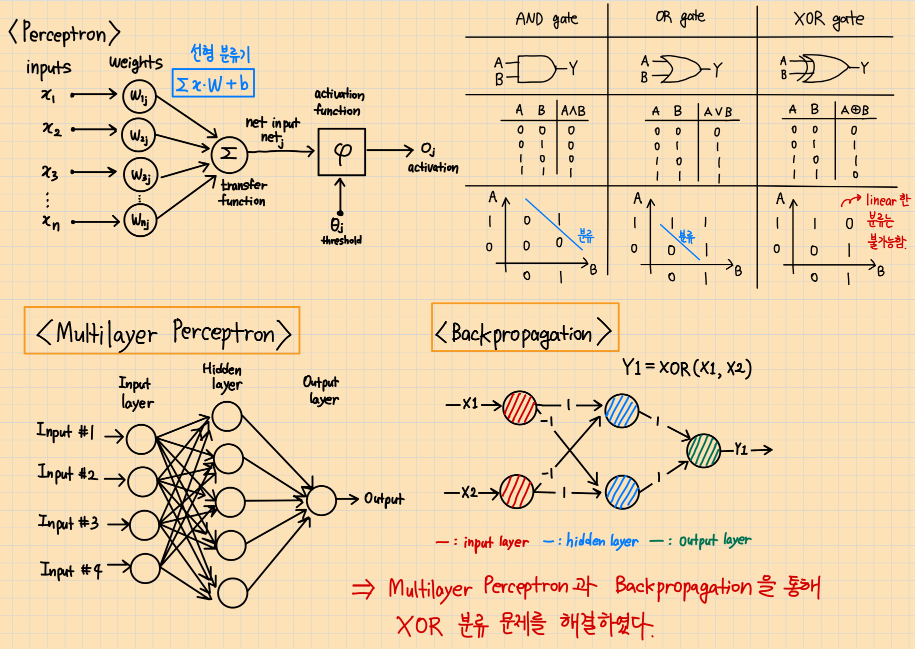
Perceptron & Multi Layer Perceptron 이론 요약

 과거에는 단일 층 퍼셉트론으로는 XOR 데이터를 분류할 수 없었지만, 다층 퍼셉트론과 역전파(Backpropagation) 알고리즘이 등장하면서 XOR 분류 문제가 해결되었다.

Perceptron & Multi Layer Perceptron 구현 코드

<Single Layer Perceptron>

라이브러리 임포트

import torch
import torch.nn as nn
import torch.optim as optim

 

XOR 단일 층 퍼셉트론 학습

# Set device
device = 'cuda' if torch.cuda.is_available() else 'cpu'

# XOR
X = torch.FloatTensor([[0, 0], [0, 1], [1, 0], [1, 1]]).to(device)
Y = torch.FloatTensor([[0], [1], [1], [0]]).to(device)

# nn Layers
linear = nn.Linear(2, 1, bias=True)
sigmoid = nn.Sigmoid()
model = nn.Sequential(linear, sigmoid).to(device)

# Cost & Optimizer definition
criterion = nn.BCELoss().to(device)
optimizer = optim.SGD(model.parameters(), lr=1)

# Training
for step in range(10001):

    # Calculate H(x) and Cost
    hypothesis = model(X)    
    cost = criterion(hypothesis, Y)
    
    # Gradient Descent
    optimizer.zero_grad()
    cost.backward()
    optimizer.step()
    
    if step % 100 == 0:
        print('Step: {:5d} Cost: {}'.format(
            step, cost.item()
        ))

 

<Multi Layer Perceptron>

라이브러리 import

# Library import
import torch

 

디바이스, XOR 데이터, 레이어, 학습률 설정

device = 'cuda' if torch.cuda.is_available() else 'cpu'

# XOR data
X = torch.FloatTensor([[0, 0], [0, 1], [1, 0], [1, 1]]).to(device)
Y = torch.FloatTensor([[0], [1], [1], [0]]).to(device)

# nn Layers
w1 = torch.randn(2, 2).to(device)
b1 = torch.randn(2).to(device)
w2 = torch.randn(2, 1).to(device)
b2 = torch.randn(1).to(device)

# Set learning rate
learning_rate = 0.5

 

시그모이드 함수, 시그모이드 미분 함수 정의

# Sigmoid function
def sigmoid(x):
    return 1.0 / (1.0 + torch.exp(-x))
    # return torch.div(torch.tensor(1), torch.add(torch.tensor(1.0), torch.exp(-x)))

# Derivative of the sigmoid function
def sigmoid_prime(x):
    return sigmoid(x) * (1 - sigmoid(x))

 

모델 학습(BCE를 통한 Cost 계산 & Backpropagation)

for step in range(10001):
    # Forward
    l1 = torch.add(torch.matmul(X, w1), b1)
    a1 = sigmoid(l1)
    l2 = torch.add(torch.matmul(a1, w2), b2)
    Y_pred = sigmoid(l2)
    
    # Binary Cross Entropy Loss
    cost = -torch.mean(Y * torch.log(Y_pred + 1e-7) + (1 - Y) * torch.log(1 - Y_pred + 1e-7))
    
    # Back propagation (Chain rule)
    # Loss derivative (Derivative of BCE)
    d_Y_pred = (Y_pred - Y) / (Y_pred * (1.0 - Y_pred) + 1e-7)
    
    # Layer 2
    d_l2 = d_Y_pred * sigmoid_prime(l2)
    d_b2 = d_l2
    d_w2 = torch.matmul(torch.transpose(a1, 0, 1), d_b2)
    
    # Layer 1
    d_a1 = torch.matmul(d_b2, torch.transpose(w2, 0, 1))
    d_l1 = d_a1 * sigmoid_prime(l1)
    d_b1 = d_l1
    d_w1 = torch.matmul(torch.transpose(X, 0, 1), d_b1)
    
    # Weight update
    w1 = w1 - learning_rate * d_w1
    b1 = b1 - learning_rate * torch.mean(d_b1, 0)
    w2 = w2 - learning_rate * d_w2
    b2 = b2 - learning_rate * torch.mean(d_b2, 0)
    
    if step % 100 == 0:
        print('Step: {:5d} Cost: {}'.format(
            step, cost.item()
        ))

실행 결과 분석

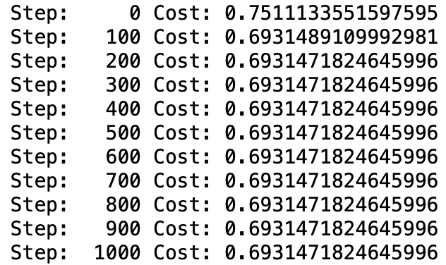
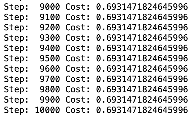
<Single Layer Perceptron>

 XOR 문제를 단일 층 퍼셉트론으로 학습한 결과 Cost가 줄어들지 않고 거의 일정한 값을 유지했다. 즉, XOR 문제는 선형적으로 분리되지 않기 때문에, 학습이 제대로 되지 않았음을 알 수 있다.

단일 층 퍼셉트론 학습 초반 / 후반

 

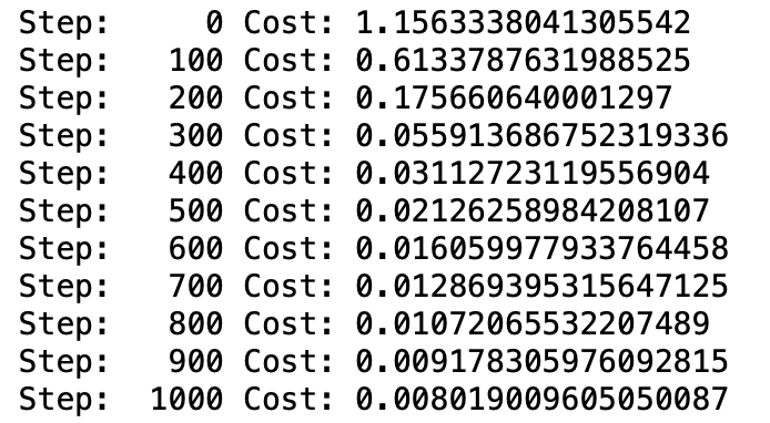
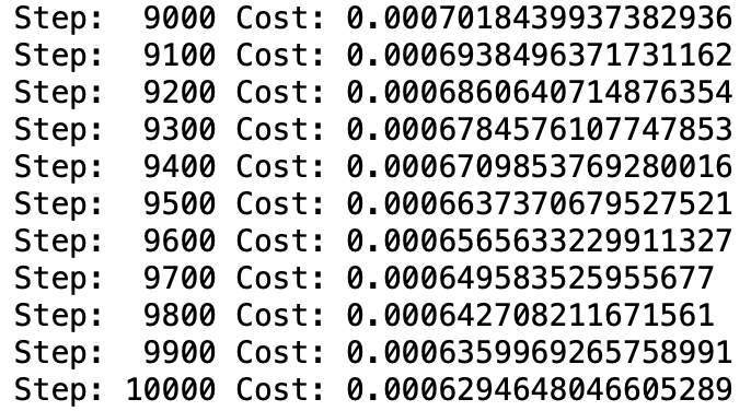
<Multi Layer Perceptron>

 Cost가 빠른 속도로 줄어들며, 학습 후반에는 약 0.0006까지 Cost 값이 줄어들었다.

다층 퍼셉트론 학습 초반 / 후반

느낀 점 

•  강의에 나온 코드대로 했는데 Cost가 NaN이 나와서 당황했다. Cost 계산식에 있는 Log 안에 너무 작은 값이 들어가서 문제가 생긴 것 같아, 작은 값인 1e-7를 더함으로써 Cost 값이 정상적으로 계산될 수 있게 했다.
• 하지만, NaN 문제를 해결한 후에는 모든 Step에 동일한 Cost가 출력되는 문제가 발생했다. 강의 코드에서는 Weight와 Bias를 설정할 때 torch.Tensor를 사용하는데, 이를 torch.randn으로 바꾸니까 Cost가 점점 감소했다. randn은 정규 분포를 따르는 난수를 생성하여 텐서를 반환하므로 안정적으로 W, b를 초기화할 수 있다.
• 학습률을 0.5로 설정하면 조금 높은 편이기는 하나, 0.1일 때보다 훨씬 빠르게 Cost가 감소해서 사용했다. 하지만, 학습률처럼 학습에 큰 영향을 미치는 하이퍼파라미터들에 대해서는 앞으로 튜닝 경험을 많이 쌓아야 할 것 같다.

 

*참고 자료

모두를 위한 딥러닝 시즌2 - Lab-08-1 Perceptron

https://youtu.be/KofAX-K4dk4?feature=shared

Lab-08-2 Multi Layer Perceptron

https://youtu.be/f-EtWNybRoI?feature=shared