[PyTorch] Train/Validation/Test & Overfitting 실습 : 모두를 위한 딥러닝 시즌2

Train/Validation/Test & Overfitting 이론 요약

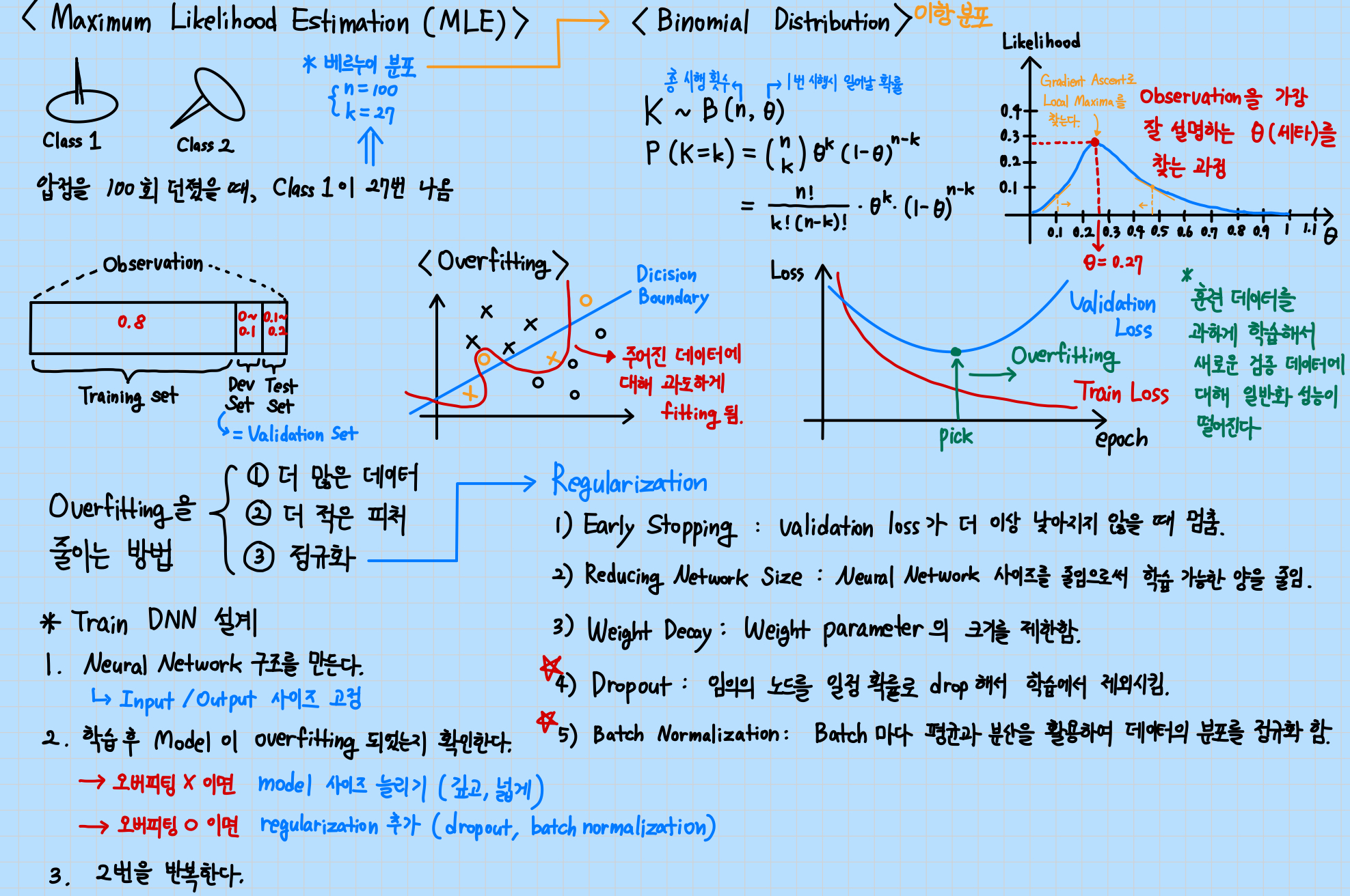
 압정을 던졌을 때 위로 떨어지는 경우를 클래스 1, 아래로 떨어지는 경우를 클래스 2로 설정한다. 총시행 횟수와 클래스 1이 나온 횟수, 1번 시행 시 일어날 확률을 사용하여 이항 분포로 모델링할 수 있다. Gradient Ascent를 통해 데이터를 가장 잘 설명하는 세타를 찾는 과정은 Likelihood를 최대화하여 Local Maxima를 찾는 과정이다.

 

 데이터를 Training set, Validation set, Test set을 일정 비율로 나누어 모델을 훈련하고 평가할 수 있다. 훈련 데이터를 과도하게 학습하는 Overfitting이 일어나면, 새로운 검증 데이터에 대해 일반화 성능이 떨어져서 Train Loss는 감소하지만, Validation Loss는 증가하는 현상을 보인다. 오버피팅을 줄이기 위해 아래 그림에 제시된 다양한 방법을 사용할 수 있다.

Train/Validation/Test & Overfitting 구현 코드

라이브러리 import & 시드값 고정

# Library import
import torch
import torch.nn as nn
import torch.nn.functional as F
import torch.optim as optim

# For reproducibility
torch.manual_seed(1)

 

Train 데이터와 Test 데이터 정의

## Data definition
# x_train = (m, 3), y_train = (m,)
x_train = torch.FloatTensor([[1, 2, 1],
                             [1, 3, 2],
                             [1, 3, 4],
                             [1, 5, 5],
                             [1, 7, 5],
                             [1, 2, 5],
                             [1, 6, 6],
                             [1, 7, 7]])
y_train = torch.LongTensor([2, 2, 2, 1, 1, 1, 0, 0])

# x_test = (m, 3), y_test = (m,)
x_test = torch.FloatTensor([[2, 1, 1], [3, 1, 2], [3, 3, 4]])
y_test = torch.LongTensor([2, 2, 2])

 

nn.Module을 상속받아 Softmax 분류 모델 클래스 정의, 모델 초기화, optimizer 정의

class SoftmaxClassifierModel(nn.Module):
    def __init__(self):
        super().__init__()
        self.linear = nn.Linear(3, 3)
    def forward(self, x):
        return self.linear(x)
    
# Initialize model
model = SoftmaxClassifierModel()

# Optimizer definition
optimizer = optim.SGD(model.parameters(), lr=0.1)

 

Train 함수 정의

# Training
def train(model, optimizer, x_train, y_train):
    nb_epochs = 20
    for epoch in range(nb_epochs):
        
        # Calculate H(x)
        prediction = model(x_train)
        
        # Calculate Cost
        cost = F.cross_entropy(prediction, y_train)
        
        # Gradient Descent
        optimizer.zero_grad()
        cost.backward()
        optimizer.step()
        
        print('Epoch {:4d}/{} Cost: {:.6f}'.format(
            epoch + 1, nb_epochs, cost.item()
        ))

 

Test 함수 정의 (Accuracy와 Cost를 계산)

# Test
def test(model, optimizer, x_test, y_test):
    prediction = model(x_test)
    predicted_classes = prediction.max(1)[1]
    correct_count = (predicted_classes == y_test).sum().item()
    cost = F.cross_entropy(prediction, y_test)
    
    print('Accuracy: {}% Cost: {:.6f}'.format(
        correct_count / len(y_test) * 100, cost.item()
    ))

 

훈련 및 테스트

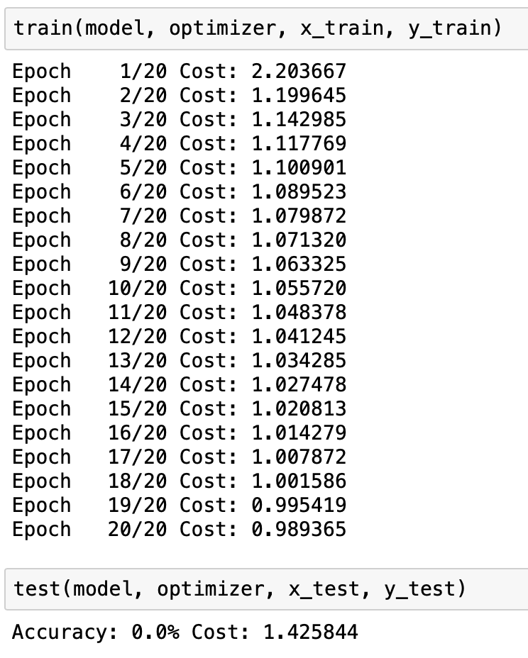
train(model, optimizer, x_train, y_train)

test(model, optimizer, x_test, y_test)

 

Learning rate에 따른 Cost 변화 관찰

# The learning rate is too large, causing the cost to diverge
model = SoftmaxClassifierModel()
optimizer = optim.SGD(model.parameters(), lr=1e5)
train(model, optimizer, x_train, y_train)

# If the learning rate is too small, the cost does not decrease
model = SoftmaxClassifierModel()
optimizer = optim.SGD(model.parameters(), lr=1e-10)
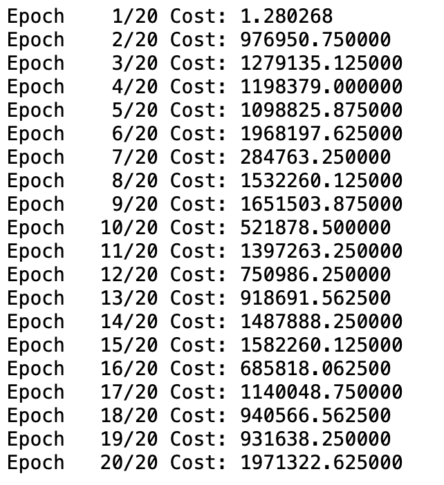
train(model, optimizer, x_train, y_train)

 

데이터 전처리 (표준화)

## Data Preprocessing
# |x_train| = (m, 3), |y_train| = (m,)
x_train = torch.FloatTensor([[73, 80, 75],
                             [93, 88, 93],
                             [89, 91, 90],
                             [96, 98, 100],
                             [73, 66, 70]])
y_train = torch.FloatTensor([[152], [185], [180], [196], [142]])

# Standardization
mu = x_train.mean(dim=0)
sigma = x_train.std(dim=0)
norm_x_train = (x_train - mu) / sigma
print(norm_x_train)

 

전처리한 norm_x_train으로 학습

# Training with Preprocessed Data
class MultivariateLinearRegressionModel(nn.Module):
    def __init__(self):
        super().__init__()
        self.linear = nn.Linear(3, 1)
        
    def forward(self, x):
        return self.linear(x)
    
# Initialize model
model = MultivariateLinearRegressionModel()

# Optimizer definition
optimizer = optim.SGD(model.parameters(), lr=1e-1)

def train(model, optimizer, x_train, y_train):
    nb_epochs = 20
    for epoch in range(nb_epochs):
        
        # Calculate H(x)
        prediction = model(x_train)
        
        # Calculate Cost
        cost = F.mse_loss(prediction, y_train)
        
        # Gradient Descent
        optimizer.zero_grad()
        cost.backward()
        optimizer.step()
        
        print('Epoch {:4d}/{} Cost: {:.6f}'.format(
            epoch + 1, nb_epochs, cost.item()
        ))
        
train(model, optimizer, norm_x_train, y_train)

실행 결과 분석

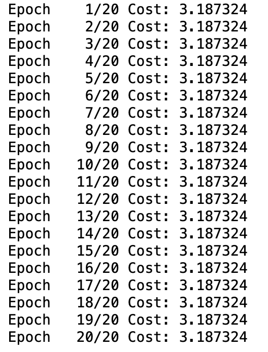
• (좌) 모델이 오버피팅으로 인해 Test 데이터에 대해 예측을 전혀 못 하는 결과가 나타났다. 
• (우) 전처리 과정에서 표준화한 데이터로 학습을 진행했을 때, 정상적으로 Cost가 감소했다. 

(좌) Train, Test 함수를 활용하여 학습 및 테스트한 결과 / (우) norm_x_train 데이터로 학습한 결과

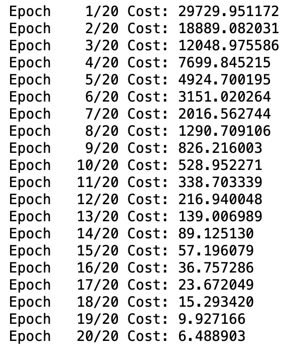
• (좌) 학습률이 너무 높으면 Cost가 점점 커지며 발산한다.
• (우) 학습률이 너무 낮으면 Cost가 줄어들지 않는다.

(좌) 학습률 = 1e5로 설정 / (우) 학습률 = 1e-10으로 설정

느낀 점

• 처음에 표준화 식을 정규화로 헷갈렸는데, 둘은 명확한 차이가 있다. 정규화는 [0, 1]과 같은 특정 범위 내로 값을 스케일링하는 방법이며, 때에 따라 다른 범위를 사용할 수도 있다. 반면, 표준화는 데이터의 평균을 0으로, 표준편차는 1로 조정하는 방법이다.
• 학습률은 일반적으로 0.1 정도로 설정하는 것 같아서 잘 바꾸지 않는 편이었다. 그런데 학습률을 매우 크거나 작게 설정했을 때 Cost 값이 직접적인 영향을 받는 것을 보니, 앞으로 모델 성능 향상을 위해 자주 튜닝하는 파라미터가 될 것 같다.

 

*참고 자료

모두를 위한 딥러닝 시즌2 - [PyTorch] Lab-07-1 Tips

https://youtu.be/JcNkszxJuak?feature=shared